(Time Series)

Recurrent Neural Networks (RNN) are among the best options for sequential data, such as text or time series. LSTM (Long Short-Term Memory) is a special type of RNN. It has the following advantages over simple RNN. LSTM;
Can prevent gradient vanishing
Can hold longer state
Can learn longer series
Can learn longer delayed relationships
In this post we will not dive deep into the mathematical details of LSTM. Instead, we will focus on implementation, starting with data preparation and ending up to examples of model code for Keras and PyTorch. But still, just for information, I would like to share the structure of LSTM below.


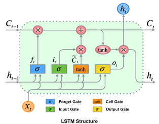

Before starting, I would like to point out that you need to scale your data except categorical features for Neural Networks kind of modelling, including Deep Learning models. Please do not forget that the weights of your Neural Network initialized randomly with small values. In addition, you must think about the the activation function you chose. It is important to consume the range of your activation function where the gradients are maximized. In the example that we will discuss in this post, we will use "tanh" as our activation function. As you can see below, the range where the gradients are maximized is [-1, 1].

So, it is a good idea to scale our data to [-1, 1] range to work around these points for maximizing the gradients, hence learning. Here is an Python example with NumPy.
import numpy as np

class MinMaxScaler:
    def __init__(self, min_value=0, max_value=1):
        if min_value >= max_value:
            raise ValueError('min_value and max_value should be set properly')
        self.min_value = min_value
        self.max_value = max_value
        self._ptp = None
        self._min = None
    def fit(self, data):
        self._ptp = np.ptp(data, axis=0).astype(np.float64)
        self._ptp[self._ptp == 0] = 1e-20
        self._min = np.min(data, axis=0)
    def transform(self, data):
        if self._ptp is None or self._min is None:
            raise RuntimeError('You should fit to data before transform')
        return (self.min_value) + ((self.max_value - self.min_value) * ((data - self._min) / self._ptp))
    def inverse_transform(self, data):
        if self._ptp is None or self._min is None:
            raise RuntimeError('You should fit to data before inverse_transform')
        return (((data - self.min_value) / (self.max_value - self.min_value)) * self._ptp) + self._min

scaler = MinMaxScaler(min_value=-1, max_value=1)
scaler.fit(X)

X_scaled = scaler.transform(X)
X_reverted = scaler.inverse_transform(X_scaled)

Scaling to [-1,1]
From this point on, we assume that our data is scaled.
Let's start modelling.
1. Data Preparation
LSTM accepts 3D data as input with shape [batch, seqence_length (seq_len), features]. For PyTorch, its default is [seq_len, batch, features], but anyway, you can set "batch_first" flag to True to use the first shape with PyTorch. Batch is a certain portion of samples as you know. Each sample is a sequence of data for LSTM and seq_len is the length of it. Features are our input values for each unit part of each sequence.
Depending on the problem but generally, we may need to approach time series and text differently from the point of data preparation, even though the math behind them is the same.
Time series data is often longer than reasonable amounts to consume as a single sequence in terms of hardware resources and learning performance as well. Keeping very long LSTM states, even if we can from the point of hardware, should be carefully evaluated. It may end up not giving enough weight to important steps in a mass environment. Thus, it may cause a decrease in performance. In addition, the importance of step values gradually decreases as they get older in most time series cases. So, setting a window size (seq_len) and moving that window over the data is a common approach for time series data.

Our data can include univariate or multivariate time series, depending on the problem that needs our solution. The picture below shows us our data source that we will use to create our dataset in this post. Each row represents a single time step. Columns are different time series and extra features as well. We can enrich our data with some extra features such as time, workday, etc. as shown. For univariate, data source is undoubtedly composed of just "Series 1" and extra features.

I prefer to add these extra features to be included in the discussions and code snippets. Better to see more details after all. If you don't need them, it is easier to remove them after you saw the big picture.
1.1. Training Dataset
In order to prepare our dataset from our source data, we will be moving over the first dimension and gather the features from the second dimension of our source data.

From data preparation perspective, the only difference for multivariate time series is to repeat the sliding window operation for each univariate time series as shown below. But at the end, we will get a dataset with the same shape [batch, seq_len, features] for both univariate and multivariate.


Important Reminder for Multivariate Time Series: Do not forget to add a distinctive identity (preferably with Embedding) to your features for each univariate time series.
Initially, we have a window of zeros. We start with the first sample to be at the end and slide the window as shown below.
Following code snippet is a Python example of creating dataset from time series data source mentioned above with sliding window for multivariate time series. "X" is input and "Y" is the target, which is next (t+1) time step value at this example. Distinctive identity (series_id) for each time series is just a number instantly generated here to be sent to the Embedding later.
def createTrainingDataset(source, window_size, num_of_series, split_ratio = 0.95):
    dataset_split_index = int(source.shape[0]*split_ratio)
    X_train_source = source[:dataset_split_index]
    X_test_source = source[dataset_split_index:]
    num_of_extra_feats = source.shape[1] - num_of_series

    # we need to create features dimension with a size of
    # num_of_extra_feats + series_id + value = num_of_extra_feats + 2

    # last Y value belongs to the window before the last
    # so, we should have one less number of windows

    X_train = np.zeros(((X_train_source.shape[0]-1)*num_of_series, window_size, num_of_extra_feats+2), dtype=np.float32)
    Y_train = np.zeros(((X_train_source.shape[0]-1)*num_of_series, 1), dtype=np.float32)
    X_test = np.zeros(((X_test_source.shape[0]-1)*num_of_series, window_size, num_of_extra_feats+2), dtype=np.float32)
    Y_test = np.zeros(((X_test_source.shape[0]-1)*num_of_series, 1), dtype=np.float32)
    window_start_position = 0
    current_window = 1
    for i in range(0, (X_train_source.shape[0]-1)*num_of_series, num_of_series):
        for series_id in range(num_of_series):
            # start series_id value from 1
            X_train[i+series_id,:,0] = series_id + 1
            X_train[i+series_id,-current_window:,1:1+num_of_extra_feats] = X_train_source[window_start_position:(window_start_position+current_window), -num_of_extra_feats:]
            X_train[i+series_id,-current_window:,-1] = X_train_source[window_start_position:(window_start_position+current_window), series_id]
            Y_train[i+series_id,0] = X_train_source[(window_start_position+current_window), series_id]
        window_start_position += (window_size == current_window) * 1
        if current_window < window_size:
            current_window += 1

    # Training dataset created. Continue with test dataset

    window_start_position = 0

    # last window of train is the first input for test
    # we can add last window of train to the head of test data

    X_test_source = np.concatenate([X_train_source[-current_window:], X_test_source], axis=0)


    for i in range(0, (X_test_source.shape[0]-1)*num_of_series, num_of_series):
        for series_id in range(num_of_series):
            # start series_id value from 1
            X_test[i+series_id,:,0] = series_id + 1
            X_test[i+series_id,-current_window:,1:1+num_of_extra_feats] = X_test_source[window_start_position:(window_start_position+current_window), -num_of_extra_feats:]
            X_test[i+series_id,-current_window:,-1] = X_test_source[window_start_position:(window_start_position+current_window), series_id]
            Y_test[i+series_id,0] = X_test_source[(window_start_position+current_window), series_id]
        window_start_position += (window_size == current_window) * 1
        if current_window < window_size:
            current_window += 1

    return X_train, Y_train, X_test, Y_test
For univariate, since you don't have a series_id anymore, you should reduce the features dimension by one, remove "for loop" of the series_id as well as the assignment line and all the references of it. Then, you will get a dataset for univariate with the same structure except series_id.
1.2. Prediction Dataset
For prediction, I prefer to start with a window full of samples rather than a window of zeros initially, so I have a slightly different creation method. However, you can go with whichever you prefer. Second difference is that we don't need to return "Y" (target) value for prediction.
def createPredictionDataset(source, window_size, num_of_series):
    num_of_extra_feats = source.shape[1] - num_of_series
    X = np.zeros(((source.shape[0]-window_size+1)*num_of_series, window_size, num_of_extra_feats+2), dtype=np.float32)
    window_start_position = 0

    for i in range(0, (source.shape[0]-window_size+1)*num_of_series, num_of_series):
        for series_id in range(num_of_series):
            X[i+series_id,:,0] = series_id + 1 # start series_id value from 1
            X[i+series_id,-window_size:,1:1+num_of_extra_feats] = source[window_start_position:(window_start_position+window_size), -num_of_extra_feats:]
            X[i+series_id,-window_size:,-1] = source[window_start_position:(window_start_position+window_size), series_id]
        window_start_position += 1

    return X
2. Model
Before starting this part, I would like to draw your attention to the feature structure of our dataset. The first column is "series_id" to be sent to Embedding. Columns, from second to last, are extra features. The last column is the value. We will create our inputs accordingly.
I would like to feed the embedding output of the series_id to the dense layer along with the LSTM. I preferred to show you two different alternatives for feeding of series_id to the embedding layer in the Keras and PyTorch examples. You can choose either of them.
For each series, we can feed the series_id value into the embedding as many as the window_size (our dataset is in this shape), so that the output will be the repetition of the same embedding result as many as the window_size, and its shape will be ready for LSTM. However, we have to take one item of embeding result to feed to the Dense layer. (PyTorch example)
For each series, we can take one item for series_id value from our dataset and feed that value into the embedding, so that the output will be one vector instead of repetition and its shape will be ready for Dense layer. However, we have to repeat this embedding output vector as many as the window_size before feeding to the LSTM. (Keras example)
Here are the draft code snippets for Keras and PyTorch to give you an idea. Details can differ according to the problem.
Keras Sample
import keras

# For Keras, "batch" dimension is not specified externally.
# It is hidden and None which means variable

# Input shape of series_id is 1 instead of window_size
# We will feed one sample for series_id

input_series_id = keras.layers.Input(shape=(1,), name='input_series_id')
input_extra_feats = keras.layers.Input(shape=(window_size, num_of_extra_feats), name='input_extra_feats')
input_series_value = keras.layers.Input(shape=(window_size, 1), name='input_series_value')
series_id_embedding = keras.layers.Embedding(input_dim=num_of_series + 1, output_dim=embedding_dim_size, name='series_id_embedding_layer')(input_series_id)
series_id_embedded = keras.layers.Flatten()(series_id_embedding)

# We need to repeat the flattened embedding values as many as
# window_size so that we can use it as an input for LSTM

features_combined = keras.layers.concatenate([keras.layers.RepeatVector(window_size)(series_id_embedded), input_extra_feats, input_series_value])

lstm1 = keras.layers.Bidirectional(keras.layers.LSTM(num_of_units, return_sequences=True, activation='tanh'))(features_combined)
drop1 = keras.layers.Dropout(0.2)(lstm1)
lstm2 = keras.layers.Bidirectional(keras.layers.LSTM(num_of_units, activation='tanh'))(drop1)
drop2 = keras.layers.Dropout(0.2)(lstm2)

# You can also feed your embedding values to the dense layer.
# Embedding is good for defining your series,
# If you don't prefer,you can directly feed "drop2" to your dense layer
# Since we fed 1 sample for series_id to embedding, output shape is
# ready for Dense. We can directly combine series_id_embedded and drop2

dense1_input = keras.layers.concatenate([series_id_embedded, drop2])
dense1 = keras.layers.Dense(dense1_out_dim, activation='tanh')(dense1_input)
dense2 = keras.layers.Dense(1, activation=None)(dense3_input)

model = keras.models.Model(inputs=[input_series_id, input_extra_feats, input_series_value], outputs=[dense2])

model.compile(optimizer=keras.optimizers.Adam(lr=learning_rate, clipvalue=clip_value), loss=keras.losses.mean_squared_error)

# Time to train.
# We will feed series_id as a single instance for each window.
# Structure of X_train mentioned above

# Training
model.fit(
 x={
 'input_series_id': X_train[:,-1:,0],
 'input_extra_feats': X_train[:,:,1:1+num_of_extra_feats],
 'input_series_value': X_train[:,:,-1:]
    },
 y=Y_train,
 validation_data=({
 'input_series_id': X_test[:,-1:,0],
 'input_extra_feats': X_test[:,:,1:1+num_of_extra_feats],
 'input_series_value': X_test[:,:,-1:]},
        Y_test
    ),
 epochs=epochs, batch_size=batch_size, shuffle=True)

# Prediction
model.predict({
 'input_series_id': X[:,-1:,0],
 'input_extra_feats': X[:,:,1:1+num_of_extra_feats],
 'input_series_value': X[:,:,-1:]},
 batch_size=batch_size)
PyTorch Sample
import torch
import torch.nn as nn
import torch.nn.functional as F
import torch.optim as optim

class Net(nn.Module):

    def __init__(self, num_of_series, num_of_features, embedding_dim_size, num_of_units):
        super(Net, self).__init__()

        self.embedding = nn.Embedding(num_of_series + 1, embedding_dim_size)

        # We will feed series_values together with extra features
        # so, LSTM input size will be
        # embedding_dim_size + num_of_features + 1

        self.lstm1 = nn.LSTM(input_size=embedding_dim_size + num_of_features + 1,
            hidden_size=num_of_units,
            num_layers=1,
            batch_first=True,
            bias=True,
            bidirectional=True,
            dropout=0.2)

        # input size of the second LSTM will be the output size of
        # the first one, which is last dimension of
        # [batch, window_size, num_directions*hidden_size]
        # whose result is "2 * num_of_units"

        self.lstm2 = nn.LSTM(input_size= 2 * num_of_units,
            hidden_size=num_of_units,
            num_layers=1,
            batch_first=True,
            bias=True,
            bidirectional=True,
            dropout=0.2)

        self.dense1 = nn.Linear(embedding_dim_size + (2 * num_of_units), dense1_out_dim)
        self.dense2 = nn.Linear(dense1_out_dim, 1)

    def forward(self, x):
        # We are feeding series_id value as many as window_size
        series_id_embedded = self.embedding(x[:,:,0])
        # output is repetition of same vector as many as window_size
        # so, shape is [batch, window_size, embedding_dim_size]
        # ready for LSTM, we can directly combine with features

        features_combined = torch.cat([series_id_embedded, x[:,:,1:]], dim=2)
        # output shape is
        #[batch, window_size, embedding_dim_size + num_of_features + 1]

        lstm1_out, _ = self.lstm1(features_combined)
        lstm1_out = F.tanh(lstm1_out)
        lstm2_out, _ = self.lstm2(lstm1_out)
        lstm2_out = F.tanh(lstm2_out)

        # We are feeding one item (last one here) of embedding output
        # to Dense layer

        dense1_input = torch.cat([lstm2_out[:,-1,:], series_id_embedded[:,-1,:]], dim=1)
        dense1_out = self.dense1(dense1_input)
        dense1_out = F.tanh(dense1_out)
        dense2_out = self.dense2(dense1_out)

        return dense2_out


# Keep data as tensor,instead of keeping same amount in memory as numpy
X_train = torch.from_numpy(X_train)
Y_train = torch.from_numpy(Y_train)

train_dataset = torch.utils.data.TensorDataset(X_train, Y_train)
train_loader = torch.utils.data.DataLoader(train_dataset, batch_size=batch_size, shuffle=True, pin_memory=True)

min_loss = float('inf')
patience_to_stop = stop_patience
total_num_of_batches = len(train_loader)

device = torch.device("cpu")
# for GPU indexed with 0 for example
# device = torch.device("cuda:0")

# Create the model
model = Net(num_of_series, num_of_features, embedding_dim_size, num_of_units)
# load model to CPU/GPU
model = model.to(device)

criterion = nn.MSELoss()
optimizer = optim.Adam(model.parameters(), lr=learning_rate)

# Training
model.train()
for epoch in range(epochs): # loop over the dataset multiple times
    running_loss = 0.0
    num_of_batches = 0
    avg_loss = 0.0

    for num_of_batches, data_pair in enumerate(train_loader, start=1):
        # get input and output from batch
        X, y = data_pair

        # load batches to CPU/GPU
        X = X.to(device)
        y = y.to(device)

        # zero the parameter gradients
        optimizer.zero_grad()

        # forward + backward + optimize
        outputs = model(X)
        loss = criterion(outputs, y)
        loss.backward()

        #clip grad params before optimizer step
        torch.nn.utils.clip_grad_norm(model.parameters(), 5)

        optimizer.step()

        # print statistics
        running_loss += loss.item()
        avg_loss = running_loss / num_of_batches

        print('\r[Epoch: %4d] [Batch: %7d/%d] loss: %.3f  ' % (epoch + 1, num_of_batches, total_num_of_batches, avg_loss), end='')
    print("") # print new line

    if avg_loss < min_loss:
        patience_to_stop = stop_patience
        min_loss = avg_loss
        torch.save(model.state_dict(), model_file_absolute_path)
    else:
        patience_to_stop -= 1
    if patience_to_stop == 0:
        break

# Prediction
model.eval()
predictions = model(X)
That's all for LSTM modelling Part 1 which is for time series data.
Hope you like it! See you in another post.