(Text)

Recurrent Neural Networks (RNN) are among the best options for sequential data, such as text or time series. LSTM (Long Short-Term Memory) is a special type of RNN. It has the following advantages over simple RNN. LSTM;
Can prevent gradient vanishing
Can hold longer state
Can learn longer series
Can learn longer delayed relationships
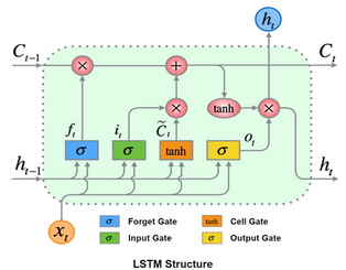
In this post we will not dive deep into the details of Embedding or math behind the LSTM. Instead, we will focus on implementation, starting with data preparation and ending up to examples of model code for Keras and PyTorch. But still, just for information, I would like to share the structure of LSTM below.


Let's start modelling.
1. Data Preparation
LSTM accepts 3D data as input with shape [batch, seqence_length (seq_len), features]. For PyTorch, its default is [seq_len, batch, features], but anyway, you can set "batch_first" flag to True to use the first shape with PyTorch. Batch is a certain portion of samples as you know. Each sample is a sequence of data for LSTM and seq_len is the length of it. Features are our input values for each unit part of each sequence.
Depending on the problem but generally, we may need to approach time series and text differently from the point of data preparation, even though the math behind them is the same.
Text is a form of data that requires a different approach than time series. A word at the beginning of a sentence or a group of sentences, which means older in the series, can have a great importance in the meaning of that text. Therefore, it would be a better approach to consider a sentence or a set of sentences as a single sequence. However, although we need to have a fixed size sequence length required for LSTM input, we have variable sequence lengths as shown below, because the sentence lengths can be variable. We will mention and solve this issue soon below.

We should start with the following steps in order.
Preprocess the text (Remove unnecessary symbols, multiple space, etc.). This part is more important for traditional Machine Learning scenarios, and gets lower importance for Deep Learning.
Dismantle your text into building blocks and assign integer ID values to them (Tokenization).
Represent these blocks as vectors in a new space where there exist built-in enrichments to define words better for LSTM (Embedding).
1.1 Tokenization
Tokenization is the secret sauce that has a significant effect on the result. There are many different studies and libraries about it such as SentencePiece (Google), Transformers (Hugging Face), etc..
Here is an example for SentencePiece.
# pip install sentencepiece

import sentencepiece as spm

# By default,
# SentencePiece uses Unknown (<unk>), BOS (<s>) and EOS (</s>)
# tokens which have the IDs of 0, 1, and 2 respectively.
# We can define an ID for padding (<pad>) as pad_id=3

spm.SentencePieceTrainer.train(input='data.txt', model_prefix='sentencepiece', vocab_size=8000, pad_id=3)

sp = spm.SentencePieceProcessor(model_file='sentencepiece.model')

# >>> sp.encode('This is a test')
# [284, 47, 11, 4, 15, 400]
# >>> sp.encode(['This is a test', 'Hello world'], out_type=int)
# [[284, 47, 11, 4, 15, 400], [151, 88, 21, 887]]
# >>> sp.encode(['This is a test', 'Hello world'], out_type=str)
# [['▁This', '▁is', '▁a', '▁', 't', 'est'], ['▁He', 'll', 'o', '▁world']]

def tokenize_with_sentencepiece(sp, file_in):
    tokens_of_text = []
    ids_of_tokens = []
    with open(file_in, 'rb') as infile:
        while True:
            line = infile.readline()
            if not line: break

            #remove new line character (\n) and convert to unicode
            line = line[:-1].decode('utf-8')

            ids_of_tokens.append(sp.encode(line))
            tokens_of_text.append(sp.encode(line, out_type=str))

    return (ids_of_tokens, tokens_of_text)

X_source_before_padding, _ = tokenize_with_sentencepiece(sp,'data.txt')
From now on, our text data has been tokenized and integer ID values have been assigned for each token. In the SentencePiece model, a dictionary of tokens and IDs is kept. We will use IDs, hereinafter referred to as tokenID, for our data source.
At this point, we should also mention the problem that sentences and therefore tokenIDs can differ in length as a sequence. However, our input shape contains a specific sequence length. We need to fix this. Taking the length of the longest sequence as our seq_len and padding the shorter ones up to that is the way to handle this. We can use the value "3" as our tokenID for padding in our case, since we have specified this value while we were creating our SentencePiece model above, so it is reserved for padding.

After tokenization and padding are done, our source data should be as follows.

Unlike time series data, the second (column) dimension of our source data as shown above defines our window size which is sequence length (seq_len). Because of padding, all samples now have the same length. Thus our seq_len is fixed.
1.2. Embedding
Embedding is the most critical concept that is the keystone of Natural Language Processing (NLP). Word2Vec, Glove, fastText, ELMo, BERT, GPT, GPT2, GPT3 are examples of important studies on word embedding.
We will not dive into the details of embedding as stated above. If you would like to learn more Embedding, you can have a look at here. However, I would like to share the logic behind it. For example, let's assume that we have trained one of the embedding models mentioned above and we can generate vectors for our tokenIDs. Let the dimension size of our embedding output space is embedding_dim.

We will use the "embed_model" as a reference to the embedding model from now on.
1.3. Training Dataset
In order to prepare out dataset from our source data, we will feed all the tokenIDs of a single row to our embedding model one by one and stack all the outputs to the first dimension as a sequence. The first row of our source data will be the first sequence (window) of our dataset with features defined by the values of embedding output vector for each tokenID.

Following code snippet is a Python example of creating dataset from text data source as shown above by simulating the embed_model as an Embedding Layer. The main idea is the same. We will map our tokenIDs to vectors. Let's assume that we are doing sentiment analysis. "X_source" is our text data source shown above with 12 different words, "X" is input (train and test) after embedding, and "Y" is the target with 3 classes, whose values can be neutral (0), positive (1) or negative (2). We will perform one-hot encoding on our target for Keras. There are many different one-hot encoder provided by frameworks and libraries, but even so, I would like to share a sample code doing one-hot encoding with Numpy. Embedding size is 3. Input size of Embedding is 13 because of starting from 1 instead of zero.

I'm aware that train and test split below is not done by considering the class density. Please take this code snippet as an example. Splitting dataset by considering the class density will be discussed in another post soon. I will put link here as soon as I published that post.
We will be using two different target "Y" for Keras and PyTorch. Because, CategoricalCrossentropy loss function of Keras expects target as one-hot encoded, whereas CrossEntropyLoss of PyTorch expects target as integer index.
One Hot Encoder for Target (Y)
def numpy_one_hot_encoder(y):
    classes = np.unique(y)
    y_encoded = np.zeros((y.shape[0], len(classes)))
    y_encoded[np.arange(y.shape[0]),[np.where(classes==_class)[0][0] for _class in y]] = 1
 return y_encoded
Source Data Simulation
>>> import numpy as np
>>>
>>> np.__version__
'1.19.1'
>>>
>>> # Simulate Text Source Data with 12 different words
>>> X_source = np.random.randint(1,13,(11,6))
>>> X_source
array([[10, 6, 2, 10, 3, 9],
 [ 4, 7, 10, 7, 9, 6],
 [ 9, 5, 1, 2, 8, 7],
 [ 7, 10, 9, 2, 8, 2],
 [10, 2, 7, 9, 2, 12],
 [10, 1, 8, 10, 11, 2],
 [ 6, 11, 11, 4, 4, 7],
 [ 2, 7, 6, 11, 7, 10],
 [ 2, 2, 4, 5, 1, 10],
 [ 6, 10, 11, 3, 7, 3],
 [ 9, 4, 1, 4, 9, 9]])
>>>
>>> X_source.shape
(11, 6)  # Shape of [samples, tokens_of_a_sequence (seq_len)]
>>>
>>> # Simulate Target Source Data with 3 different class
>>> # positive, negative and neutral
>>> Y_source = np.random.randint(0,3,(11,))
>>>
>>> Y_source
array([1, 1, 1, 0, 1, 0, 2, 2, 1, 2, 1])
>>>
>>> Y_source.shape
(11,)
Keras sample
>>> import keras
>>>
>>> keras.__version__
'2.4.3'
>>>
>>> embed_model = keras.layers.Embedding(input_dim=13, output_dim=3)
>>>
>>> X = embed_model(keras.backend.constant(X_source))
>>> X.shape
TensorShape([11, 6, 3])
>>>
>>> X = X.numpy()
>>> X.shape
(11, 6, 3)  # Shape of [batch, seq_len, features]
>>>
>>> X
array([[[-0.03160626, 0.02309431, 0.02509064],
 [ 0.04069556, -0.00658255, -0.00572851],
 [ 0.00816143, 0.03980586, -0.00733942],
 [-0.02230144, -0.00589595, -0.00962845],
 [ 0.04069556, -0.00658255, -0.00572851],
 [ 0.04319907, 0.03173921, -0.04520426]],

 [[-0.0440869 , 0.02157461, -0.03423224],
 [ 0.04069556, -0.00658255, -0.00572851],
 [ 0.04319907, 0.03173921, -0.04520426],
 [ 0.04069556, -0.00658255, -0.00572851],
 [ 0.01481513, -0.03078004, -0.02531953],
 [ 0.00816143, 0.03980586, -0.00733942]],
 .
 .
 .
 .
 [[ 0.00816143, 0.03980586, -0.00733942],
 [-0.02230144, -0.00589595, -0.00962845],
 [-0.02230144, -0.00589595, -0.00962845],
 [-0.0440869 , 0.02157461, -0.03423224],
 [-0.0440869 , 0.02157461, -0.03423224],
 [ 0.04069556, -0.00658255, -0.00572851]]], dtype=float32)
>>>
>>> # Shuffle X and Y_source in unision
>>> # along first axis to split as train and test
>>> n_elems = X.shape[0]
>>> indicies = np.random.choice(n_elems, size=n_elems, replace=False)
>>>
>>> X = X[indicies]
>>> Y = Y_source[indicies]
>>>
>>> dataset_split_index = int(X.shape[0]*split_ratio)
>>>
>>> X_train = X[:dataset_split_index]
>>> X_test = X[dataset_split_index:]
>>> Y_train = numpy_one_hot_encoder(Y[:dataset_split_index])
>>> Y_test = numpy_one_hot_encoder(Y[dataset_split_index:])
PyTorch Sample
>>> import torch
>>>
>>> torch.__version__
'1.6.0'
>>>
>>> embed_model = torch.nn.Embedding(num_embeddings=13, embedding_dim=3)
>>>
>>> X = embed_model(torch.from_numpy(X_source))
>>> X.shape
torch.Size([11, 6, 3])
>>>
>>> X = X.cpu().detach().numpy()
>>>
>>> X.shape
(11, 6, 3)  # Shape of [batch, seq_len, features]
>>>
>>> X
array([[[ 0.27464947, -0.8911431 , 0.09539263],
 [ 1.1958091 , -0.19036123, -1.4163382 ],
 [ 0.8554373 , 1.255636 , 1.1653287 ],
 [ 0.27464947, -0.8911431 , 0.09539263],
 [ 0.72696763, -0.547744 , -1.5570897 ],
 [ 0.7732037 , 1.5421947 , -0.98831576]],

 [[ 0.1104815 , 0.49442995, -0.41749394],
 [ 0.17696765, -0.05844537, -0.19660667],
 [ 0.27464947, -0.8911431 , 0.09539263],
 [ 0.17696765, -0.05844537, -0.19660667],
 [ 0.7732037 , 1.5421947 , -0.98831576],
 [ 1.1958091 , -0.19036123, -1.4163382 ]],
 .
 .
 .
 .
 [[ 0.7732037 , 1.5421947 , -0.98831576],
 [ 0.1104815 , 0.49442995, -0.41749394],
 [-0.09197728, 0.81196016, -1.2153981 ],
 [ 0.1104815 , 0.49442995, -0.41749394],
 [ 0.7732037 , 1.5421947 , -0.98831576],
 [ 0.7732037 , 1.5421947 , -0.98831576]]], dtype=float32)
>>>
>>> # Shuffle X and Y_source in unision
>>> # along first axis to split as train and test
>>> n_elems = X.shape[0]
>>> indicies = np.random.choice(n_elems, size=n_elems, replace=False)
>>>
>>> X = X[indicies]
>>> Y = Y_source[indicies]
>>>
>>> dataset_split_index = int(X.shape[0]*split_ratio)
>>>
>>> X_train = X[:dataset_split_index]
>>> X_test = X[dataset_split_index:]
>>> Y_train = Y[:dataset_split_index]
>>> Y_test = Y[dataset_split_index:]
1.2. Prediction Dataset
Preparation of predict dataset is the same as the preparation of the training dataset. The only difference is that we don't need to return "Y" values.
2. Model
I would like to share draft code snippets for Keras and PyTorch to give you an idea. Details can differ according to the problem.
For multiclass classification problems, pushing the softmax activation into the loss function significantly simplfies the computation and increases the numerical stability. Because of that, we will not use any activation function at the output of our model and we will feed the scores (logits) to the loss function instead of post-softmax probability distributions. PyTorch's CrossEntropyLoss expects logits by default. You can use CategoricalCrossentropy loss function of Keras with "from_logits=True" parameter to do this.
Keras Sample
import keras

# For Keras, "batch" dimension is not specified externally.
# It is hidden and None which means variable

input_seq = keras.layers.Input(shape=(seq_len, embedding_dim), name='input_seq')

lstm1 = keras.layers.Bidirectional(keras.layers.LSTM(num_of_units, return_sequences=True, activation='tanh'))(input_seq)
drop1 = keras.layers.Dropout(0.2)(lstm1)
lstm2 = keras.layers.Bidirectional(keras.layers.LSTM(num_of_units, activation='tanh'))(drop1)
drop2 = keras.layers.Dropout(0.2)(lstm2)

dense1 = keras.layers.Dense(dense1_out_dim, activation='tanh')(drop2)
dense2 = keras.layers.Dense(3, activation=None)(dense3_input)

model = keras.models.Model(inputs=[input_seq], outputs=[dense2])

model.compile(optimizer=keras.optimizers.Adam(lr=learning_rate), loss=keras.losses.CategoricalCrossentropy(from_logits=True))

# Training
model.fit(
 x={'input_seq': X_train},
 y=Y_train,
 validation_data=({'input_seq': X_test}, Y_test),
 epochs=epochs, batch_size=batch_size, shuffle=True)

# Prediction
model.predict({'input_seq': X}, batch_size=batch_size)
PyTorch Sample
import torch
import torch.nn as nn
import torch.nn.functional as F
import torch.optim as optim

class Net(nn.Module):

    def __init__(self, embedding_dim_size, num_of_units):
        super(Net, self).__init__()

        self.lstm1 = nn.LSTM(input_size=embedding_dim_size,
            hidden_size=num_of_units,
            num_layers=1,
            batch_first=True,
            bias=True,
            bidirectional=True,
            dropout=0.2)

        # input size of the second LSTM will be the output size of
        # the first one, which is last dimension of
        # [batch, window_size, num_directions*hidden_size]
        # whose result is "2 * num_of_units"

        self.lstm2 = nn.LSTM(input_size= 2 * num_of_units,
            hidden_size=num_of_units,
            num_layers=1,
            batch_first=True,
            bias=True,
            bidirectional=True,
            dropout=0.2)

        self.dense1 = nn.Linear(2 * num_of_units, dense1_out_dim)
        self.dense2 = nn.Linear(dense1_out_dim, 3)

    def forward(self, x):
        lstm1_out, _ = self.lstm1(x)
        lstm1_out = F.tanh(lstm1_out)
        lstm2_out, _ = self.lstm2(lstm1_out)
        lstm2_out = F.tanh(lstm2_out)

        dense1_out = self.dense1(lstm2_out[:,-1,:])
        dense1_out = F.tanh(dense1_out)
        dense2_out = self.dense2(dense1_out)

        return dense2_out


# Keep data as tensor,instead of keeping same amount in memory as numpy
X_train = torch.from_numpy(X_train)
Y_train = torch.from_numpy(Y_train)

train_dataset = torch.utils.data.TensorDataset(X_train, Y_train)
train_loader = torch.utils.data.DataLoader(train_dataset, batch_size=batch_size, shuffle=True, pin_memory=True)

min_loss = float('inf')
patience_to_stop = stop_patience
total_num_of_batches = len(train_loader)

device = torch.device("cpu")
# for GPU indexed with 0 for example
# device = torch.device("cuda:0")

# Create the model
model = Net(embedding_dim_size, num_of_units)
# load model to CPU/GPU
model = model.to(device)

criterion = nn.CrossEntropyLoss()
optimizer = optim.Adam(model.parameters(), lr=learning_rate)

# Training
model.train()
for epoch in range(epochs): # loop over the dataset multiple times
    running_loss = 0.0
    num_of_batches = 0
    avg_loss = 0.0

    for num_of_batches, data_pair in enumerate(train_loader, start=1):
        # get input and output from batch
        X, y = data_pair

        # load batches to CPU/GPU
        X = X.to(device)
        y = y.to(device)

        # zero the parameter gradients
        optimizer.zero_grad()

        # forward + backward + optimize
        outputs = model(X)
        loss = criterion(outputs, y)
        loss.backward()

        optimizer.step()

        # print statistics
        running_loss += loss.item()
        avg_loss = running_loss / num_of_batches

        print('\r[Epoch: %4d] [Batch: %7d/%d] loss: %.3f  ' % (epoch + 1, num_of_batches, total_num_of_batches, avg_loss), end='')
    print("") # print new line

    if avg_loss < min_loss:
        patience_to_stop = stop_patience
        min_loss = avg_loss
        torch.save(model.state_dict(), model_file_absolute_path)
    else:
        patience_to_stop -= 1
    if patience_to_stop == 0:
        break

# Prediction
model.eval()
predictions = model(X)
That's all for LSTM modelling Part 2 which is for text data.
Hope you like it! See you in another post.